4.5.4 回归项-分位数损失(Quantile Loss)
迭代公式:
图像:
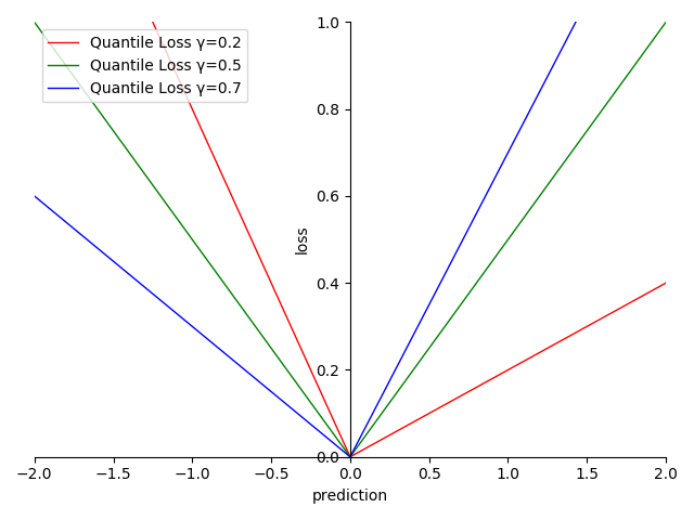
图 4-27 Quantile Loss 函数图
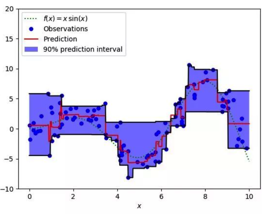
图 4-28 Quantile Loss 样本拟合示意图
特性:
- 当预测值残差在 时,梯度为设定值
- 当预测值残差在 时,梯度为设定值
- 可通过 的设定,来有指向的调整模型结果, 的可范围在
- 适用于区间预测,通过调整 范围覆盖预测区间
- 非光滑(non-smooth)
- 非指数计算,算力消耗相对较低
分位数损失(Quantile Loss) 是一种用于区间预测的损失函数。MAE、MSE、Huber 等损失函数,基于的是最小二乘法,默认预测实际值残差方差保持不变且相对独立。而以分位数损失作为损失函数的回归模型,对于具有变化方差或非正态分布的残差,也能给出合理的预测区间。
分位损失函数中, 值代表对预测结果的预判程度: 值 越大,对结果被低估的惩罚程度越高,即越容易被 高估 ; 值 越小,对结果被高估的惩罚程度越高,即越容易被 低估。在区间预测过程中,通过调整 取值范围,来实现对样本的覆盖,得到预测区间。
因为 Quantile Loss 的这种特性,常被用来做商业评估类型的回归模型。
Quantile Loss 算子化
利用 C 语言实现对算子的封装,有:
#include <math.h>
#include <stdio.h>

double quantile_loss(double *y_true, double *y_pred, int size, double q) {
  double sum = 0;
  for (int i = 0; i < size; i++) {
    double error = y_true[i] - y_pred[i];
    if (error > 0) {
      sum += q * error;
    } else {
      sum += (1 - q) * error;
    }
  }
  return sum / size;
}

int main() {
  int size = 3;
  double y_true[] = {0.5, 0.75, 1.0};
  double y_pred[] = {0.6, 0.8, 0.9};
  double q = 0.5;
  double quantile_loss_value = quantile_loss(y_true, y_pred, size, q);
  printf("The quantile loss is %f\n", quantile_loss_value);
  return 0;
}
运行验证可得到结果:
The quantile loss is 0.083333