3.3.2 朴素目标检测结果度量 - IoU & GIoU
考虑到算法本身需要作为目标检测结果准确性的衡量标准,并用于模型的计算过程。所以不能采用较高复杂程度的算法。而 交并比(IoU [Intersection over Union]) 计算作为相对简单的区域检测算法,则是可被采用的不错方案。
交并比顾名思义,即为交集和并集的比值。 只不过这里的交集和并集,指的是 预测结果(Prediction)对应的预测框(Anchor Box)和标注框(Ground Truth)的交集与并集,记为 和 。
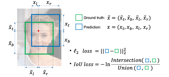
图 3-11 原论文中交并比示意图[19]
如图所示,交并比公式非常简洁(注意 并非 IoU Loss ),可记为:
而根据交并比设计的损失函数,就是交并比损失函数(IoU Loss)。
同其他有关深度学习领域,针对损失函数提出的算法理论一致。IoU Loss 在模型中同样存在两项应用,分别为 前向预测(Forward Prediction) 和 反向传播(Backward Propagation)。 即标准损失的计算和模型梯度迭代的加速。
交并比损失函数(IoU Loss)
根据原论文的设计,IoU 前向扩散作用在 ReLU 激活函数层(ReLU Layer)后,以代替传统物体识别模型采用的 损失函数,判断待筛选的预测框是否命中。由于始终有 ,交并比损失函数可被认为是 的 特殊交叉熵损失函数(cross-entropy Loss),有:
带入交并比实际值,有:
此即为 交并比损失函数。由于 有 ,考虑到计算便利性,在条件范围内常用差值代替对数计算。即:
相比 损失函数的简单区域差值来衡量命中的方式, IoU 考虑到了 预测框与标准框的平面空间位置关系,并通过对位置的衡量 锁定了两者间的平面位姿独立优化,因而具有更贴合客观的代表性。且在交叉熵类型损失函数(详见下一章)的特性作用下,结果落于单位量化的百分比区间,利于阈值衡量和操作之便。
交并比损失函数(IoU Loss)的反向传播(Backward Propagation)
反向传播(Backward Propagation) 简单来说,是通过当前学习到的参数在参数空间内指定方向的运动趋势,来反相强化或衰减该方向上的参数权重,进而达到更快使模型拟合的数学方法论统称。自 杰弗里·辛顿(Geoffrey Hinton,“深度学习之父”,当代人工智能领域三巨头之一) 教授提出并汇总这一概念以来,持续的被作为深度学习根基理论之一,应用在各类算法的学习过程中。
如果从物理学角度来看,把参与训练的相关模型参数的权重向量比作速度,那么,损失函数的反向传播,就相当于 速度在各个方向上的某一时刻的加速度。所以,其影响的是权重在方向上的迭代步长变化,即为优化算法的输出。
交并比损失函数的反向传播,为便于称呼,简称 反向交并比(Backward IoU/ IoU Back)。取图 3.3.2-1 说明,记预测框为 面积为 ,标注框为 面积为 ,则反向交并比可表示为:
其中, 是 预测框面积关于位置的偏导数(Partial Derivative), 是 交集区域面积关于位置的偏导数,有:
带入求得 值,作用于 优化算法的梯度变换,如 自适应动量算法(Adam) 等。来发挥相应作用。
交并比损失函数(IoU Loss)的简单 C++ 语言实现
到这里,我们就可以根据基本情况来做一下交并比的代码实现了。由于需要进行一些基本的矩阵运算,我们选择采用引入 轻量级的 GLM(GL Mathematics) 开源库,来协助完成基本工作。
我们选择 GLM 库的原因,是因为其可以通过纯粹的包含头文件的方式,简便轻巧的启动包含基本图形矩阵数据结构和方法的完整库功能。在其开源协议保证下,非常适合运用于大部分工程项目。如果需要也可以自己分装部分算法和操作。例如在某些场景下,我们需要计算物体体积方块区域,到视窗平面上的投影位置:
#include <glm/ext.hpp>

#include "stdio.h"
#include "math.h"

typedef glm::vec2 Vector_2f;
typedef glm::vec3 Vector_3f;
typedef glm::vec4 Vector_4f;
typedef glm::mat2 Matrix_2x2f;
typedef glm::mat3 Matrix_3x3f;
typedef glm::mat4 Matrix_4x4f;

#define XC_PI 3.14159265358979323846
#define XC_RADIAN(d_) (XC_PI * d_ / 180.0f)
#define XC_VECTOR_NORMALIZE(v_) glm::normalize(v_)
#define XC_VECTOR_CROSS(vl_, vr_) glm::cross(vl_, vr_)
#define XC_VECTOR_DOT(vl_, vr_) glm::dot(vl_, vr_)
#define XC_MATRIX_INVERSE(m_) glm::inverse(m_)
#define XC_MATRIX_TRANSPOSE(m_) glm::transpose(m_)
#define XC_MATRIX_DOT(ml_, mr_) dot_m4x4(ml_, mr_)
#define XC_V4_M44_DOT(vl_, mr_) dot_v4_m4x4(vl_, mr_)

Vector_4f
dot_v4_m4x4(Vector_4f v4_, Matrix_4x4f m4x4_) {
    return m4x4_[0] * v4_[0] + m4x4_[1] * v4_[1] + m4x4_[2] * v4_[2] + m4x4_[3] * v4_[3];
}

Matrix_4x4f
dot_m4x4(Matrix_4x4f ml_, Matrix_4x4f mr_) {
    Matrix_4x4f result_;
    result_[0] = mr_[0] * ml_[0][0] + mr_[1] * ml_[0][1] + mr_[2] * ml_[0][2] + mr_[3] * ml_[0][3];
    result_[1] = mr_[0] * ml_[1][0] + mr_[1] * ml_[1][1] + mr_[2] * ml_[1][2] + mr_[3] * ml_[1][3];
    result_[2] = mr_[0] * ml_[2][0] + mr_[1] * ml_[2][1] + mr_[2] * ml_[2][2] + mr_[3] * ml_[2][3];
    result_[3] = mr_[0] * ml_[3][0] + mr_[1] * ml_[3][1] + mr_[2] * ml_[3][2] + mr_[3] * ml_[3][3];
    return result_;
}
此处我们简单的实现了两个快速算法,用于协助我们完成目标 向量与 矩阵的点乘,和两个 矩阵的点乘。 其实类似的快速算法已在库内有封装,此处仅是用于说明 GLM 的一些基本用法。
不过,对于交并比的代码工程化来说,并不需要这么复杂:
#include <glm/ext.hpp>

#include "stdio.h"
#include "math.h"

typedef glm::vec2 Vector_2f;
typedef glm::vec4 Vector_4f;

bool static IoU_simple(Vector_4f anchor_box_, Vector_4f ground_box_, float threshold_ = 0.8f) {
    float M_area_, T_area_, I_area_, U_area_;
    float IoU_mark_;
    {
        Vector_2f I_lt = {
            MAX(anchor_box_[0], ground_box_[0]),
            MAX(anchor_box_[1], ground_box_[1])
        };
        Vector_2f I_rb = {
            MIN(anchor_box_[2], ground_box_[2]),
            MIN(anchor_box_[3], ground_box_[3])
        };
        if (I_rb.x < I_lt.x || I_rb.y < I_lt.y) {
            return false;
        }
        M_area_ = MAX(ABS(anchor_box_[2] - anchor_box_[0]), 0) *
                  MAX(ABS(anchor_box_[3] - anchor_box_[1]), 0);
        T_area_ = MAX(ABS(ground_box_[2] - ground_box_[0]), 0) *
                  MAX(ABS(ground_box_[3] - ground_box_[1]), 0);
        I_area_ = MAX(ABS(I_lt.x - I_rb.x), 0) * MAX(ABS(I_lt.y - I_rb.y), 0);
        U_area_ = M_area_ + T_area_ - I_area_;
        IoU_mark_ = I_area_ / U_area_;
    }
    return (1 - IoU_mark_ > threshold_);
}
上面的简短过程,就是整个交并比的 C++ 语言封装了。可见易于迁移。
IoU 的缺点与 GIoU 的改进
交并比损失函数并非是没有缺陷的。 一个显而易见的问题就是 IoU 无法评估预测框和标注框无交集区域时,预测框的优劣程度(梯度消失)。 这所造成的直接问题就是,当 无交集情况出现,我们将无法只通过 IoU 损失函数,来使预测框快速的向标注框方向运动。从而导致数据浪费并产生不准确的结果,且有可能使模型陷入局部解而导致停滞。
2019 年的 CVPR 上,来自斯坦福大学的研究团队以交并比为基础,提出了 IoU 的改进版 通用交并比(GIoU [Generalized Intersection over Union])算法 [20] 。解决了无交集的判断问题。
GIoU 采用的处理办法为,在原有 IoU 计算的基础上,引入预测框与标注框区域所构成的最小外接矩形,即 两者的最小外接闭包(smallest enclosing convex) 参与损失函数计算,来辅助量化两者之间的远近到权重迭代中, 记为 。
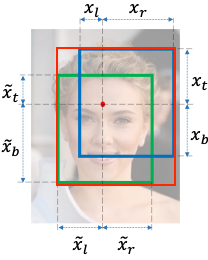
图 3-12 红框即为 IoU 图例中,I 和 U 的最小外接矩形
改进后的通用交并比公式 同样非常简洁 (注意 并非 GIoU Loss ),可记为:
从公式可知,当 预测框与标注框不存在交集时, 有:
当 预测框与标注框完全重合时, 有:
基于此,GIoU 的取值范围为 。
通用交并比损失函数(GIoU Loss)
GIoU 本质是一种对 IoU 算法的 泛化补充,所以在损失函数 的表达上,直接采用 GIoU 代替 IoU 作为影响因子即可。有:
同理,记 是预测框面积关于位置的偏导数(Partial Derivative), 是标注框面积关于位置的偏导数(Partial Derivative), 是交集区域面积关于位置的偏导数,有:
而 标注框在单次迭代中是常量值,即 代入:
显然 GIoU 的反向传播计算相比 IoU 更为快捷有效。这也是其 通用性 的体现之一。
通用交并比损失函数(GIoU Loss)的简单 C++ 语言实现
万事具备,现在只需要代码实现 GIoU 算法即可,仍然非常便捷。只需在原 IoU 算法上补充改进部分即可:
#include <glm/ext.hpp>

#include "stdio.h"
#include "math.h"

typedef glm::vec2 Vector_2f;
typedef glm::vec4 Vector_4f;

bool static GIoU_simple(Vector_4f anchor_box_, Vector_4f ground_box_, float threshold_ = 0.8f) {
    float M_area_, T_area_, I_area_, U_area_, C_area_;
    float IoU_mark_, GIoU_mark_;
    {
        Vector_2f I_lt = {
            MAX(anchor_box_[0], ground_box_[0]),
            MAX(anchor_box_[1], ground_box_[1])
        };
        Vector_2f I_rb = {
            MIN(anchor_box_[2], ground_box_[2]),
            MIN(anchor_box_[3], ground_box_[3])
        };
        if (I_rb.x < I_lt.x || I_rb.y < I_lt.y) {
            return false;
        }
        M_area_ = MAX(ABS(anchor_box_[2] - anchor_box_[0]), 0) *
                  MAX(ABS(anchor_box_[3] - anchor_box_[1]), 0);
        T_area_ = MAX(ABS(ground_box_[2] - ground_box_[0]), 0) *
                  MAX(ABS(ground_box_[3] - ground_box_[1]), 0);
        I_area_ = MAX(ABS(I_lt.x - I_rb.x), 0) * MAX(ABS(I_lt.y - I_rb.y), 0);
        U_area_ = M_area_ + T_area_ - I_area_;
        IoU_mark_ = I_area_ / U_area_;
    }
    {
        Vector_2f C_lt = {
            MIN(anchor_box_[0], ground_box_[0]),
            MIN(anchor_box_[1], ground_box_[1])
        };
        Vector_2f C_rb = {
            MAX(anchor_box_[2], ground_box_[2]),
            MAX(anchor_box_[3], ground_box_[3])
        };
        if (C_rb.x < C_lt.x || C_rb.y < C_lt.y) {
            return false;
        }
        C_area_ = MAX(ABS(C_lt.x - C_rb.x), 0) * MAX(ABS(C_lt.y - C_rb.y), 0);
        GIoU_mark_ = IoU_mark_ - (C_area_ - U_area_) / C_area_;
    }
    return ((1.0 - GIoU_mark_) * 0.5f > threshold_);
}
完成 GIoU 算法的程序化封装。
GIoU 的缺点与 IoU 算法族的发展
那么,GIoU 算法是否依旧存在缺陷呢?
虽然 GIoU 可以适度的缓解无交集情况的梯度消失问题,但 并不能加速当预测框完整包含标注框时的梯度迭代。此时 GIoU 算法,会因为最小外接矩形等同于并集 的缘故,退化为 IoU 算法。从而无法起到有向加速梯度趋向更贴合标注大小的目的。
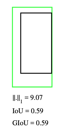
图 3-13 预测框(绿)包含标注框时 GIoU 退化为 IoU 示意图[20]
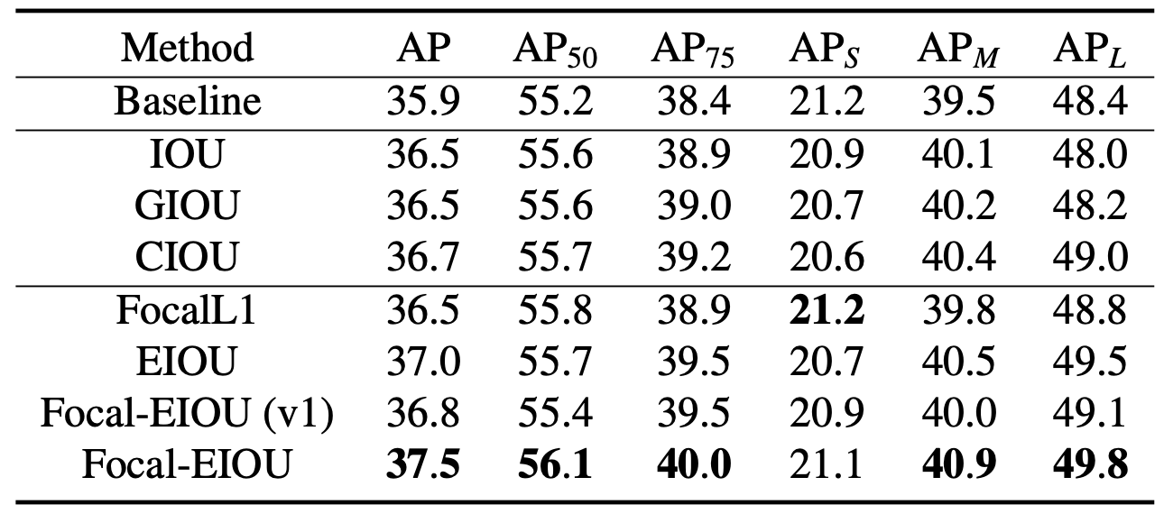
针对这种情形,后续的一些研究试图通过引入 框中心点(DIoU [Distance-IoU]) [21] ,结合 长宽一致性(CIoU [Complete-IoU]) [21] ,并在中心点基础上 进一步优化损失函数的设计(EIoU [Efficient-IoU]) [22] 来解决此问题。虽然取得了不错的效果,但算法复杂度也有较大变化,考虑到实际工程情况取舍可以酌情选用,本书不再展开讲解。
几种算法的对比结果如表 《当前主流 IoU 算法族基于 COCO val-2017 数据集的对比结果》 所示 [22],仅供参考:
进行到这里,在一些耗时训练之后,我们就能够得到一个静态的物体识别算法模型了。 由于静态模型不需要持续迭代,通过直接取模型参数或者接入其他成型的推理引擎,即可完成对指定关注物体的识别操作。
需要注意的是,目前训练所得的 简易模型,还不能在 不经过辅助方法 的情况下,自主完成锁定需要检测的物体。模型只能用于判断某一个给定检测范围(检测框)内的数据,是否属于被用于训练录入的标签物体,并给出命中率。
因此,依旧需要人为提供用于辅助锁定检测目标的方法。 配合检测所得命中率经过阈值筛选最终结果,得到其所处像素位置。